As shown in Figure 4-3 on the "Plasma Experiments" page, various types of measurements are utilized in plasma experiments to clarify detailed physical properties. Among these diagnostic methods, our laboratory focuses on developing interferometry and Thomson scattering diagnostics. Both methods employ light sources that emit electromagnetic waves, such as lasers or microwave sources. Methods that inject electromagnetic waves or particle beams from the outside are called "active diagnostics," while methods that measure light emission or radiation from the plasma itself are called "passive diagnostics." Active diagnostics can increase the signal intensity by utilizing powerful sources, whereas the signal strength of passive diagnostics is entirely determined by the state of the plasma. However, active diagnostics require the preparation of light sources or particle beams in addition to detectors, doubling the effort needed to set up the measurement system. Furthermore, active diagnostics have advanced hand-in-hand with the historical development of electromagnetic wave sources and particle beams.
5-1. Interferometry
Interferometers are widely used not only in plasma diagnostics but also in many fields of physical measurement. Historically famous examples include the Michelson-Morley experiment, which verified the constancy of the speed of light, and more recently, the detection of gravitational waves. Both measured minute changes in position. An interferometer is a measurement technique based on the superposition (interference) of light waves. If two waves of the same intensity meet, they reinforce each other when their crests align (constructive interference) and cancel each other out when a crest meets a trough (destructive interference).
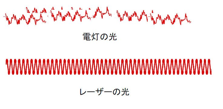
While interferometry can be performed using any light source in principle, it is not easily achieved with the standard electric lamps used in daily life. Figure 5-1 shows a comparison between light from an electric lamp and laser light. The horizontal axis of Figure 5-1 can represent either the spatial or temporal axis. Light from a lamp contains various wavelengths, and its waves are fragmented spatially and temporally. This means that even a small distance away or a short time later, the wave loses any relation to its original state. This inability to maintain a spatial or temporal relationship is referred to as being spatially and temporally uncorrelated, or "incoherent." In contrast, laser light has a single wavelength, and its phase relationship is strictly maintained over time and space, making interferometry straightforward. A state where the phase relationship is preserved spatially and temporally is called "coherent." Strictly speaking, lasers come in many types, and maintaining a long coherence length and coherence time requires sophisticated stabilization control. Simple lasers not designed for interferometry, such as the semiconductor lasers used in common laser pointers, do not possess long coherence lengths or times.
Next, let us explain the mechanism of an interferometer using Figure 5-2. As shown in Figure 5-2(a), light enters from the left. The light is split by a half mirror (beamsplitter), which reflects half of the light and transmits the rest. The reflected light travels toward Mirror 1, and the transmitted light travels toward Mirror 2. The light waves reflected back from Mirror 1 and Mirror 2 recombine at the half mirror, mixing together. Half of this combined light then proceeds to the detector.
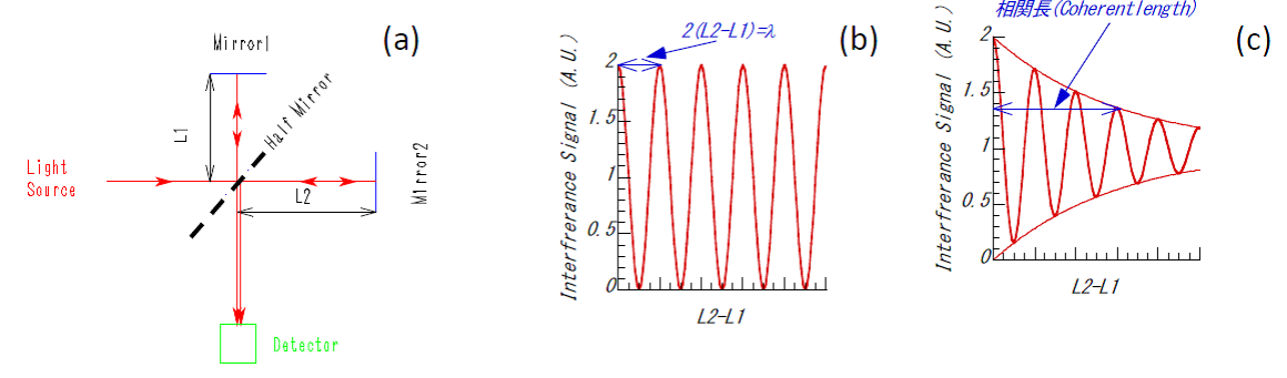
Here, by moving Mirror 1 or Mirror 2, we can alter the distances $L_1$ or $L_2$ from the half mirror to each respective mirror. When twice the difference between $L_1$ and $L_2$ is an integer multiple of the source wavelength, the light waves constructively interfere. When it is an odd multiple of a half-wavelength, they destructively interfere. We consider twice the distance difference because, in the interferometer shown in (a), the light travels back and forth between the half mirror and the mirrors, meaning the light propagates twice the distance the mirror is moved. When a coherent laser is used, the interference signal oscillates as the mirror moves, as shown in Figure 5-2(b). However, if an incoherent light source like a lamp is used, an interference signal can only be obtained when the distance difference is extremely small (on the order of the light's coherence length). As the distance difference grows, the interference signal quickly vanishes, as shown in Figure 5-2(c). Before the advent of lasers in the 1960s, interferometry was performed using lamps or atomic emission lines, which required an extraordinarily strict alignment to match the lengths of the two paths exactly.
What exactly can an interferometer measure in plasma experiments? The answer is electron density. As discussed on the "What is Nuclear Fusion" and "Plasma Experiments" pages, it is the hydrogen ions that undergo fusion reactions. However, directly measuring ion density is technically challenging. Therefore, most experiments utilize the electron density per unit volume (typically per $\text{cm}^3$ or $\text{m}^3$) as an indicator of plasma density—essentially, how "thick" the plasma is. Unlike measuring voltage, current, or resistance with a multi-tester, most plasma diagnostic methods cannot directly measure the desired quantity. For instance, the wavelength and intensity of light emitted from a plasma depend on a complex mixture of electron temperature, electron density, ion temperature, and fuel gas density, making it difficult to isolate and evaluate these parameters from emission alone. On this point, interferometry holds a major advantage: once the wavelength of the light source is known, the measured phase shift is determined uniquely by the electron density within the plasma.
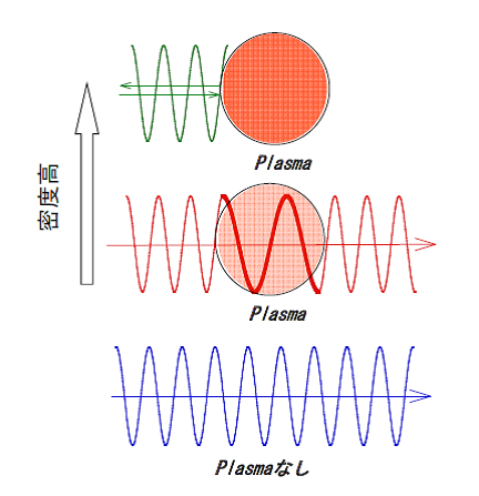
How do we measure electron density? We exploit the property that the wavelength of light (electromagnetic waves) changes in proportion to the electron density as it passes through a plasma. Figure 5-3 illustrates the behavior of an electromagnetic wave injected into a plasma. Compared to a vacuum, the wavelength of the electromagnetic wave becomes longer inside the plasma. This is mathematically equivalent to shortening the effective spatial length of the path. This effective spatial length shortens in direct proportion to the electron density. Therefore, when plasma exists along the path of the interferometer beam, as shown in Figure 5-3, it produces the exact same effect as physically moving one of the mirrors.
An interferometer measures the difference in optical path length (the distance traveled by the light from the source to the detector) between the two arms. The fact that the waves reinforce each other when the path difference is an integer multiple of the wavelength, and cancel when it is an odd multiple of a half-wavelength, means that constructive interference occurs when the phase difference between the two paths is $2\pi n$, and destructive interference occurs when it is $\pi(n + 1/2)$ (where $n = 0, 1, 2, \dots$). Naturally, for any phase values in between, a combination of these effects occurs. The total phase shift $\Delta\phi$ including all states is given by the following equation. For the derivation of this formula, please refer to Reference [12].
 (5-1)
Here, $\lambda$ is the laser wavelength in meters ($\text{m}$), $\bar{n}_e$ is the average electron density in the plasma in $\text{m}^{-3}$, and $L$ is the path length through the plasma in meters ($\text{m}$).
If the electron density rises even higher, the wavelength approaches infinity, at which point the electromagnetic wave is completely reflected. As a familiar example, a layer of plasma called the ionosphere exists high in Earth's atmosphere, and it reflects radio waves up to around $50\,\text{MHz}$. Today, overseas communication relies on fiber-optic cables and satellites, but more than 50 years ago, long-distance wireless communication relied heavily on reflecting electromagnetic waves off the ionosphere.
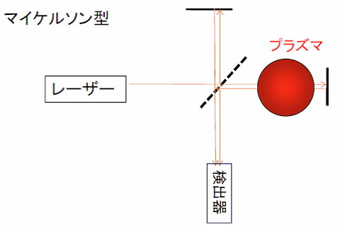
Figure 5-2 illustrates a Michelson interferometer. Another common configuration is the Mach-Zehnder interferometer shown in Figure 5-5, where the laser beam is split and travels along two separate paths before interfering. The Michelson type requires fewer mirrors and allows the light to pass through the plasma twice (back and forth), doubling the measured phase shift caused by the electron density. However, a drawback of the Michelson type is that reflected light can travel back into the laser cavity, potentially destabilizing the laser oscillation.
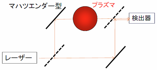
Now, let us discuss the signal processing of interferometers in more detail. Figure 5-6 shows the typical signals observed during a plasma discharge. As discussed on the "Plasma Experiments" page, a plasma discharge begins with breakdown (ignition), followed by fuel gas injection to increase the density. The density is kept constant by adjusting the gas puff, and finally, the density decays at the end of the discharge. A schematic of this density evolution over time is shown in Figure 5-6(b). When the plasma is generated, a phase shift occurs between the light path passing through the plasma (probe path) and the path that does not (reference path), because the wavelength lengthens inside the plasma, as shown in Figure 5-6(a). The resulting interference signal is shown in Figure 5-6(c). During the density rise and decay phases, the phase difference changes over time (corresponding to moving the mirror in Figure 5-2), producing a series of fringes (alternating bright and dark signals). However, when the density becomes constant, the interference signal also becomes stationary. When the density decreases, the fringe patterns reappear. Mathematically, the interference signal can be described by Equation (5-2), where $E_p$ is the amplitude of the light passing through the probe path and $E_r$ is the amplitude of the light passing through the reference path.
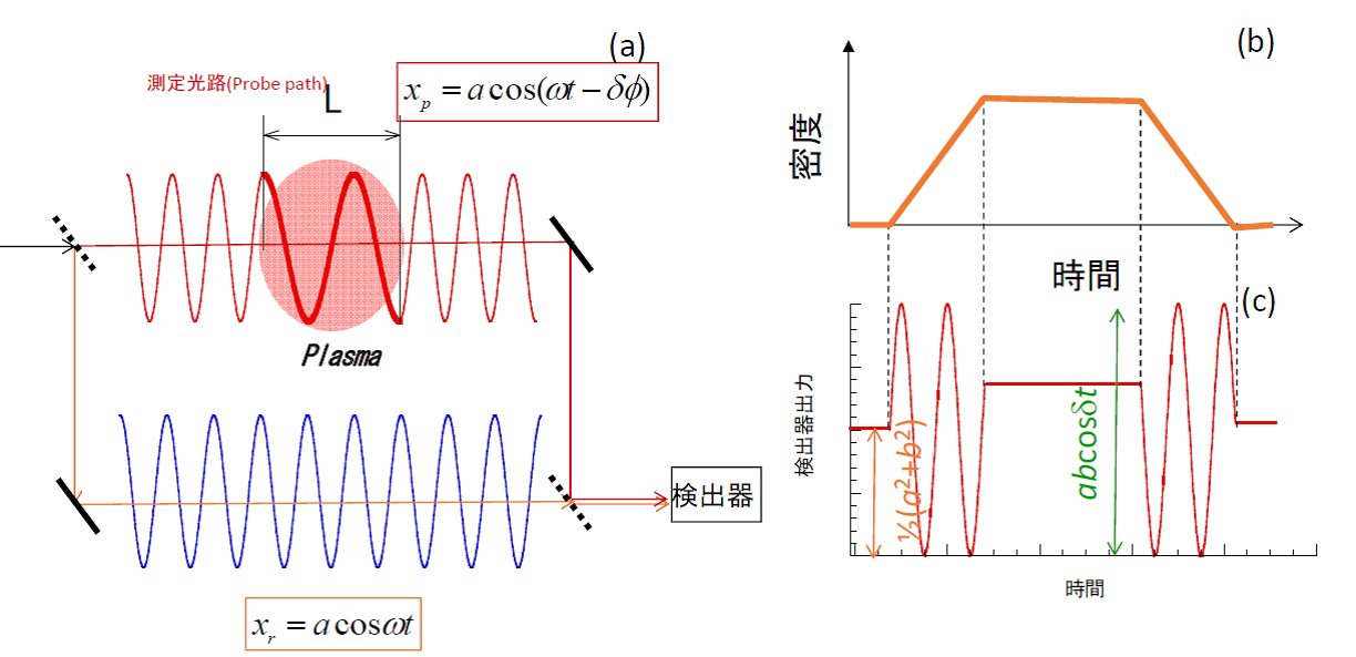
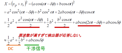
In Equation (5-2), note that the terms involving $\omega t$ or $2\omega t$ oscillate at frequencies far too high for the optical detector to respond to, so they average out to zero and do not contribute to the measured signal. As a result, the recorded interference signal takes the form of a cosine wave. This configuration is called "homodyne detection." The term $\Delta\phi$ in the cosine wave corresponds to the phase shift given by Equation (5-1). While Equation (5-1) is a direct function of the electron density (specifically, the line-integrated density), accurately calculating the exact phase shift from a simple cosine wave is challenging. This is especially true when the total phase shift is less than one full fringe (i.e., $\Delta\phi < 2\pi$), because the signal is non-linear with respect to the phase change, making highly precise measurements difficult.
To overcome this limitation and measure phase shifts of less than $2\pi$ with high precision, plasma interferometry widely employs a method called "heterodyne detection." Figure 5-7 shows the heterodyne detection system and its signal outputs. The setup in Figure 5-7(a) is considerably more complex than the homodyne system in Figure 5-6(a). The key feature of this method is the use of a frequency shifter to slightly shift the frequency of one of the laser beams. Mixing and detecting these two slightly different frequencies creates a "beat frequency" (or intermediate frequency), which acts as a carrier wave for the measurement. Heterodyne detection requires two detectors: one records the beat signal between the reference beam and the probe beam that passed through the plasma, while the other records the beat signal between the reference beam and an unperturbed beam. The resulting signals are described by Equations (5-3) and (5-4). Again, the extremely high-frequency $\omega t$ terms are filtered out by the detector response. The beat frequency is chosen to match the operational range of the detectors and electronics, typically ranging from $10\,\text{kHz}$ to $50\,\text{MHz}$ in plasma diagnostics. Several methods are used to shift the frequency, such as using two separate lasers with slightly different wavelengths (twin lasers), using an acousto-optic modulator (AOM) where acoustic waves interact with the light inside a crystal, or using a rotating diffraction grating disk that shifts the frequency of the reflected light via the Doppler effect.
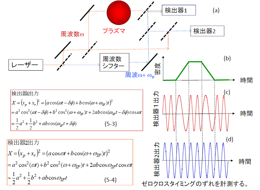
The beat signal from Detector 2, which combines beams that did not pass through the plasma, provides a steady reference wave as shown in Figure 5-7(d). On the other hand, the beat signal from Detector 1 combines the shifted reference beam with the probe beam, yielding a wave that contains the plasma-induced phase shift $\Delta\phi$ within its phase component, as shown in Figure 5-7(c). Comparing the waveforms from Detector 1 and Detector 2, the timing of their zero-crossings differs because of the phase shift term $\Delta\phi$. By measuring this time delay between the two signals, the phase shift can be determined. Since this time delay varies linearly with the phase shift, heterodyne detection allows for exceptionally high-precision measurements.
On the LHD, three separate heterodyne interferometers are installed. The first is a millimeter-wave interferometer (wavelength $\lambda \approx 1\,\text{mm}$) used as the main electron density monitor. The second is a multi-channel far-infrared (FIR) laser interferometer ($\lambda = 119\,\mu\text{m}$) dedicated to measuring electron density profiles. The third is a carbon dioxide ($\text{CO}_2$) laser interferometer ($\lambda = 10.6\,\mu\text{m}$), which acts as a high-density diagnostic to prevent signal loss when the plasma density exceeds the measurement threshold of the FIR system.
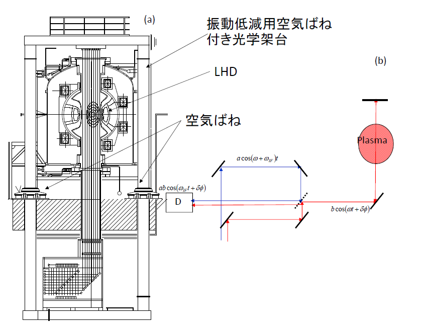
Figure 5-8(a) shows the 13-channel FIR laser interferometer system on the LHD. As illustrated in Figure 3-4 on the "Large Helical Device" page, the interferometer is positioned to span across the doughnut-shaped vacuum vessel. The laser beams are transmitted from the diagnostic diagnostic room located next to the LHD torus hall. They are split into 14 channels on a massive optical framework supported by air-spring dampers; 13 channels pass through the plasma volume inside the vacuum vessel, while the remaining channel serves as an external reference path. The entire optical frame is isolated on air springs because the mechanical vibrations from vacuum pumps and nearby machinery generate severe phase noise that must be mechanically damped.
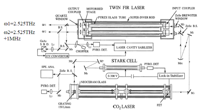
The schematic layout of the system is shown in Figure 5-8(b). The laser beams injected into the vacuum vessel pass completely through the plasma, reflect off internal mirrors, and pass back through the plasma again, forming a Michelson configuration that doubles the phase shift effect. The light source consists of a dual-cavity "twin" laser system, where $\text{CO}_2$ pump lasers excite alcohol vapor inside two glass tubes, producing two FIR wavelengths with a stable frequency separation of $1\,\text{MHz}$ to generate the heterodyne beat signal. Figure 5-9 shows this specialized laser system, which was developed through long-term collaborative research by Professor Okajima's group at Chubu University and Professor Kawahata's group at NIFS (both are currently Professors Emeriti).
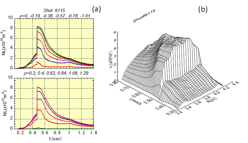
Figure 5-10 shows an example of the electron density measurements obtained with the FIR interferometer. At $0.45\,\text{seconds}$, the density spikes rapidly; this is caused by the injection of a solid hydrogen ice pellet, which abruptly fuels the core plasma. It is vital to remember that the interferometer measures the line-integrated density along the path of each laser cord. The cross-section of the plasma consists of nested, concentric layers as shown in the center of the vacuum vessel in Figure 5-8(a). These nested layers are called "magnetic surfaces." Because the electron density and most other physical parameters are uniform along any given magnetic surface, a mathematical inversion technique called "Abel inversion" is required to reconstruct the local electron density profile from the 13 line-integrated datasets. The reconstructed spatial distribution of the electron density over time is shown in Figure 5-10(b). In the early phase of the discharge, the profile exhibits a hollow center, but immediately following the pellet injection, it transitions into a highly peaked profile with an elevated core density. Analyzing these dynamic profile variations allows us to understand the underlying nature of electron particle transport. For those interested in a deeper look, you can download "Plasma Summer School - Particle Transport in Magnetically Confined Plasmas.pdf" from our "Lectures & Presentations" page.
5-2. Thomson Scattering Diagnostics
Thomson scattering diagnostics are perhaps the most widely implemented and vital tools for physical analysis in the field of magnetically confined plasmas. The scattering of electromagnetic radiation can be broadly divided into scattering by neutral particles and scattering by charged plasma particles. Examples of the former include Mie scattering and Rayleigh scattering. Mie scattering occurs when electromagnetic waves interact with neutral particles that are larger than the wavelength of the light, such as sunlight scattering off cloud droplets or headlights scattering through thick fog. Sunlight contains many wavelengths, but clouds appear white because all visible wavelengths are scattered equally. Rayleigh scattering describes the interaction of light with particles much smaller than the wavelength, such as oxygen and nitrogen molecules in the atmosphere. Rayleigh scattering is strongly dependent on wavelength, with shorter wavelengths scattering far more efficiently. The blue color of the sky during the day and the deep red of sunrises and sunsets are direct consequences of this wavelength dependence; blue light has a shorter wavelength than red light, so it scatters throughout the atmosphere, making the sky appear blue. Why then is the sun red at dawn and dusk? At these times, the sun is positioned at a low angle near the horizon, forcing the sunlight to travel through a much longer path of the atmosphere to reach our eyes. Along this extended path, the blue light is scattered away entirely, leaving only the unscattered red light to pass through. The moon can appear reddish near the horizon for the exact same reason.
In contrast, Thomson scattering involves the interaction of electromagnetic waves with free electrons within a plasma. Since it never occurs in daily life, it can be a bit difficult to conceptualize. We will briefly explain its principles here, but for rigorous derivations, please consult References [7], [8], [9], and [15].
While Mie and Rayleigh scattering can be observed using standard ambient sunlight or standard headlights without extreme intensity or focus, Thomson scattering diagnostics require an exceptionally high-intensity laser source. Thomson scattering is categorized into two regimes: "incoherent Thomson scattering" (often referred to as non-collective) and "collective Thomson scattering" (CTS). Incoherent Thomson scattering measures electron temperature and electron density, while collective Thomson scattering measures bulk ion temperature, ion density, and plasma waves. Typically, when researchers in the nuclear fusion community say "Thomson scattering" without qualification, they are almost always referring to incoherent Thomson scattering. This is because incoherent Thomson scattering is standard equipment on nearly all major plasma devices, whereas collective Thomson scattering setups for evaluating ion dynamics are exceedingly rare worldwide.
Figure 5-11 compares the underlying physical principles of incoherent and collective Thomson scattering.
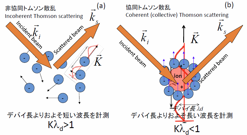
In Figures 5-11(a) and (b), the blue dots represent electrons and the red dots represent ions. As shown in Figure 5-11(a), electrons and ions move around randomly due to thermal motion. However, if we look closer at individual ions as shown in Figure 5-11(b), a fundamental property of plasma is its tendency to maintain macroscopic electrical neutrality. Consequently, electrons gather around each ion to shield its positive charge. When an ion moves, this cloud of shielding electrons moves along with it, resulting in a coordinated, collective motion. While individual electrons move completely randomly at microscopic scales, when viewed at a slightly larger scale (greater than the plasma Debye length), they move collectively, tracking the thermal motion of the ions. Because electromagnetic waves are scattered almost entirely by the light electrons rather than the heavy ions (even the lightest hydrogen ion is roughly 1,800 times heavier than an electron, meaning its response to the light's electric field is negligibly small), observing scattering at small scales reveals the electron temperature and density, while observing at larger, collective scales reveals the ion temperature and density. Consider Figure 5-12: imagine a swan swimming gracefully across a quiet lake. The swan generates ripples on the water's surface as indicated by the blue lines. Even if the swan itself were invisible, we could accurately deduce its movement and velocity simply by observing the ripples. Collective Thomson scattering operates on this exact logic: the target of the measurement is the thermal motion of the ions, but we measure it by observing the collective ripples they induce in the electron cloud.
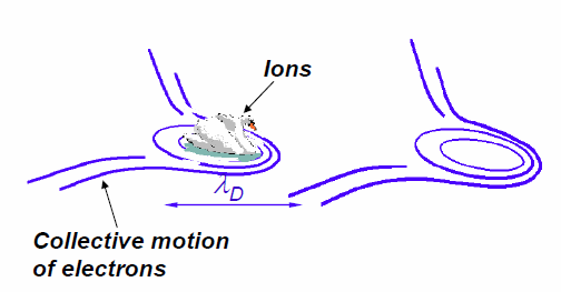
(Image courtesy of Dr. Søren Korsholm, Technical University of Denmark.)
By the way, while "collective" translates directly to "集団的" (group-like) in Japanese, the pioneers of laser diagnostics in Japan chose to translate it as "協同" (cooperative) Thomson scattering, capturing how particles cooperate to act as a system. Conversely, the regime involving independent electron motion was translated as "非協同" (non-cooperative / incoherent). In English, "incoherent" was selected as the antonym for collective, but since a direct translation like "無相関" (uncorrelated) sounds awkward in Japanese, the early pioneers opted for "非協同トムソン散乱." I find these translations possess an elegant linguistic flair, reminiscent of how Masaoka Shiki masterfully translated "baseball" into the poetic Japanese word "野球" (Yakyu) rather than a rigid literal translation.
Figure 5-13 shows a schematic overview of an incoherent Thomson scattering system. An exceptionally powerful laser pulse must be injected into the plasma; today, Q-switched pulsed Nd:YAG lasers are the gold standard. Unlike continuous-wave lasers used in common laser pointers, pulsed lasers emit their total energy in ultra-short bursts, allowing them to achieve the immense peak power required for scattering. Current Nd:YAG lasers used in diagnostics can fire between 30 to 100 pulses per second. Because the immense power generates significant thermal load on the laser crystals, the pulse repetition rate is strictly limited by cooling requirements. As shown in Figure 5-13, the laser pulse is focused into the plasma volume and scatters off the thermally moving electrons. Though the incident laser light has a single, razor-sharp wavelength, the scattered light undergoes a Doppler shift due to the rapid thermal motion of the electrons, broadening the spectrum. A higher electron temperature results in a broader scattered spectrum, allowing the temperature to be determined directly from the spectral width. Meanwhile, the absolute intensity of the scattered light is linearly proportional to the electron density. However, because the absolute scattered intensity is easily affected by laser power fluctuations, alignment drift, and detector degradation, an independent calibration experiment is required to establish the absolute density. This calibration is typically performed by filling the vacuum vessel with a known pressure of nitrogen gas and measuring its Rayleigh scattering intensity. Since this calibration is technically demanding, researchers sometimes fix the shape of the profile using the Thomson data and scale its absolute magnitude so that its line-integral matches the data from the independent laser interferometer diagnostic.
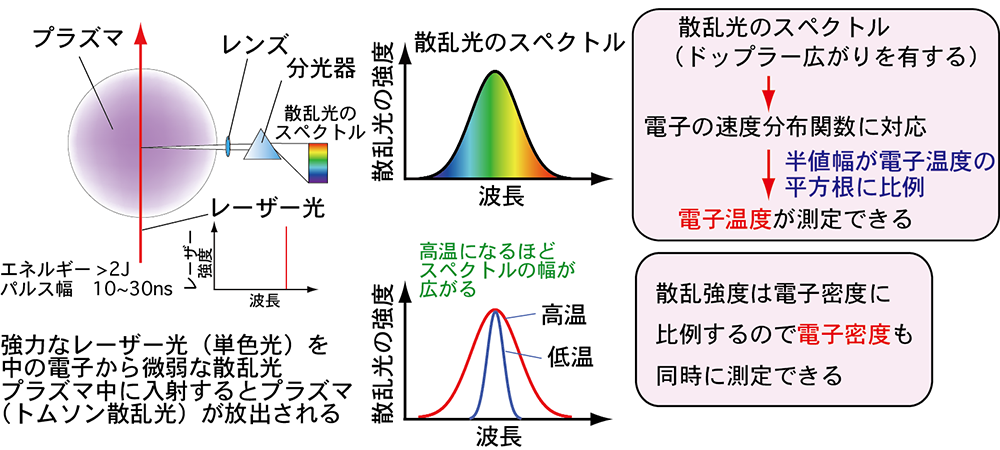
(Image courtesy of Dr. Toshifumi Hatae, National Institutes for Quantum Science and Technology.)
Figure 5-14 shows the historic incoherent Thomson scattering system deployed on a Russian tokamak in 1969. This diagnostic system and its results confirmed the breakthrough performance achieved on the T-3 tokamak device at the Kurchatov Institute in 1968, as referenced in Table 3-1 on the "Large Helical Device" page.

(b) Circles: plasma current of $40\,\text{kA}$, Crosses: $60\,\text{kA}$, Squares: $85\,\text{kA}$ [2]
At that time, high-repetition-rate YAG lasers operating at 30–100 Hz had not yet been invented, so a ruby laser was utilized as the light source. Ruby lasers remained the mainstay of Thomson scattering diagnostics until about 20 years ago. Although they fired extremely high-energy pulses, their intense cooling requirements limited their firing rate to roughly one pulse per minute. This specific system was developed by team members from the Culham Laboratory in the UK, who traveled to the Kurchatov Institute in the USSR with their equipment to perform the measurements during the height of the Cold War. As shown in Figure 5-14(b), the scattered spectrum clearly broadens as the plasma current is increased. The measured core temperature of $1000\,\text{eV}$ ($11.6\,\text{million Kelvin}$) was only about one-tenth of the temperature required for a commercial reactor, but it was an astonishing milestone for that era. Even today, many modern mid- and small-scale experimental devices operate routinely around $1000\,\text{eV}$. These definitive diagnostic results proved that the tokamak configuration could reach temperatures far exceeding any other confinement concepts of the time, prompting fusion laboratories worldwide to pivot almost instantly toward tokamak research. This stands as a historic example of how a single diagnostic measurement completely altered the course of fusion energy history.
Figure 5-15 shows the modern YAG Thomson scattering system currently operating on the LHD. This advanced system measures local electron temperature and density simultaneously across 200 distinct spatial points. While the historic T-3 setup measured light scattered at a 90-degree angle, the LHD system cannot accommodate a 90-degree viewing port due to the presence of the massive superconducting helical coils. Instead, it is configured to collect backscattered light returning along a path close to the incident laser axis. The collected light is transmitted to detectors via a large bundle of optical fibers. By combining four 50-Hz lasers and three 10-Hz lasers, the system can measure profiles at a maximum rate of $100\,\text{Hz}$. By fine-tuning the trigger timing between the individual laser units, it is also possible to record rapid transient phenomena with a time resolution of less than $1\,\text{ms}$ for short durations. This diagnostic system has operated reliably since the LHD began experiments in 1998.
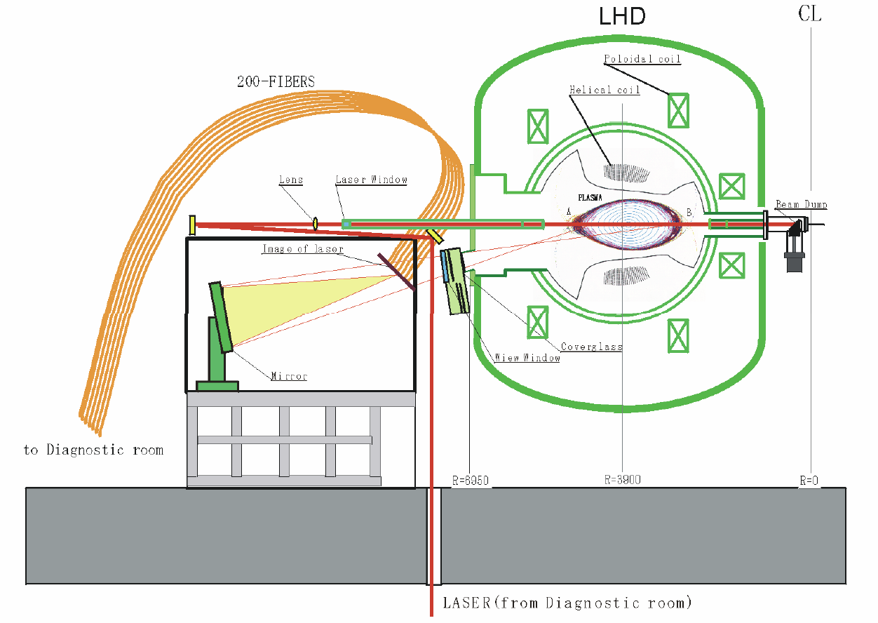
Figure 5-16 shows an example of data recorded by this diagnostic. Before the LHD YAG Thomson system went online, most Thomson scattering diagnostics worldwide were limited to around 10 to 20 spatial points. Systems utilizing ruby lasers combined with CCD cameras could capture more than 100 points, but their low repetition rate meant they could not track temporal evolution during a single discharge. The LHD system revolutionized this by providing both high spatial resolution and continuous temporal tracking. As shown in Figure 5-16, the electron temperature profile does not always form a perfectly smooth curve; it can flatten out in localized regions as seen in (a), or develop a localized, steep temperature gradient as seen in (b).
The details of our collective Thomson scattering system will be introduced on the "Research" page. With the diagnostic principles covered here, let us now proceed to explore the specific research projects being pursued in our laboratory. Please move on to the "Research" page from the top menu.
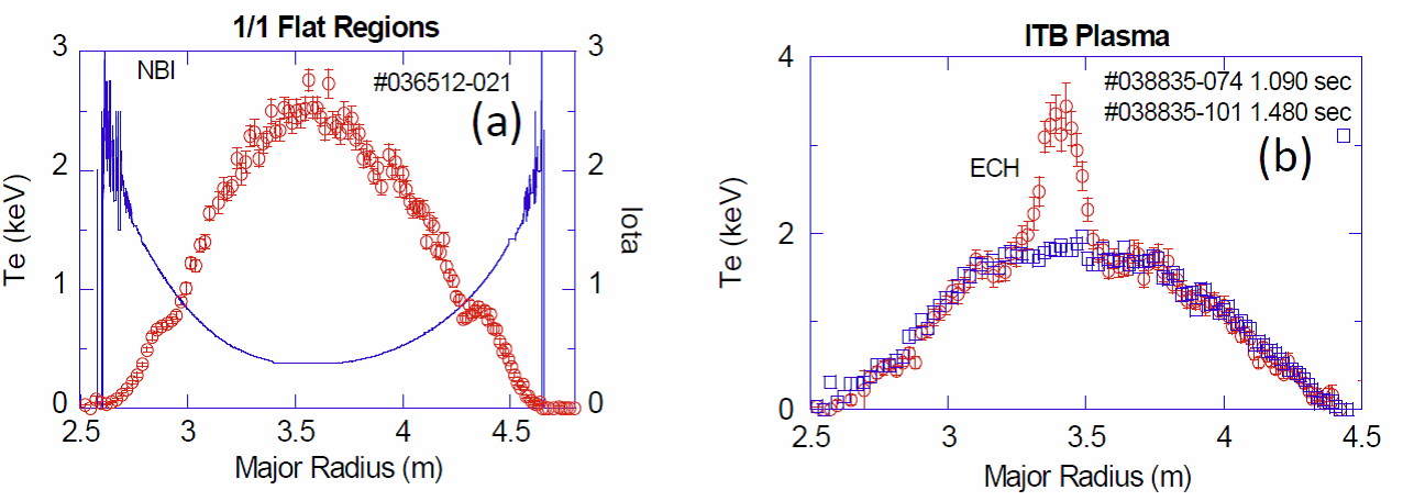
Red circles: Electron temperature, Blue squares: Electron density, Blue solid line: Rotational transform
(Image courtesy of Dr. Ichihiro Yamada, National Institute for Fusion Science.)
References
- F.F. Chen, (Translated by T. Uchida), "Introduction to Plasma Physics", Maruzen (1977)
- K. Kawahata, K. Tanaka, Y. Ito, A. Ejiri, and S. Okajima, “Far infrared laser interferometer system on the Large Helical Device”, Review of Scientific Instruments, Vol. 70 (1999), pp.707-709
- Kenji TANAKA, Kazuo KAWAHATA, Tokihiko TOKUZAWA, Shigeki OKAJIMA, Yasuhiko ITO, Katsunori MURAOKA, Ryuichi SAKAMOTO, Kiyomasa WATANABE, Tomohiro MORISAKI, Hiroshi YAMADA and the LHD Experimental group, “Density Reconstruction Using a Multi-Channel Far-Infrared Laser Interferometer and Particle Transport Study of a Pellet-Injected Plasma on the LHD”, Plasma and Fusion Research, Vol. 3 (2008) pp. 050-1-050-15
- Dustin H. Froula, Siegfried Glenzer, Neville C. Luhmann Jr., John Sheffield, “Plasma Scattering of Electromagnetic Radiation Theory and Measurement Technique 2nd Edition”, ELSEVIER, Academic Press
- I. YAMADA, K. NARIHARA, H. FUNABA, T. MINAMI, H. HAYASHI, T. KOHMOTO, “RECENT PROGRESS OF THE LHD THOMSON SCATTERING SYSTEM”, FUSION SCIENCE AND TECHNOLOGY, Vol. 58, JULY/AUG. (2010), 345